Using Probability Theory to Benefit the Company

Updated for Lethal Company version 65!

Lethal Company is a “co-op horror game about scavenging at abandoned moons to sell scrap to the Company.”¹ In the game, you (and up to 3 of your friends) take an autopilot spaceship to several dangerous planets in order to collect scrap items which you can sell to your enigmatic employer, only referred to as The Company. The catch is these planets are the home of several monsters or entitites which will promptly dispatch of unsuspecting scavengers who invade their territory.

The Company’s terrible totally legal™ and ethical™ business model relies on its employees completing a sequence of profit quotas which they must fulfill in the span of 3 days. Each time you complete a quota, the next quota will be higher. That is, every 3 days there is an increasing amount of profit you must achieve if you don’t want the company to promptly dispatch of you very violently fire you with a modest compensation package. This blog post is sponsored by The Company.

In this post, I’d like to jump head-first into the inner workings of how the quota system works and see if we can derive some useful mathematical results from it.

This post delves somewhat deeply into some mathematical topics which may not be straightforward to understand. Even I am just trying to learn them! If you’d like to join me in this endeavour, go ahead and read the entire post. If not, feel free to skip to the Results section at the end!

A Quick Lesson in Probability Theory

What Even Is Randomness, Anyway?

Imagine you’re flipping a fair coin. How many things can happen?

1. The coin lands on Heads;
2. The coin lands on Tails.

Those are our only two possible outcomes. Now, what are the chances that each of these actually happens? Intuitively, we know that if we have a fair coin then it’s a 50/50 chance of it landing on Heads or Tails… but how do we formalise this mathematically?

Let’s try “inventing” a way to do this. Say we have a letter $X$ which we define to denote our concept of outcome. Next, let’s assign a number to each outcome. For simplicity, let’s say “1” for when our coin lands on Heads, and “2” for when our coin lands on Tails.

Using this, we can express formulae for concepts like “The probability that the coin lands on Tails is 50%”, which becomes $Pr(X=2)=1/2$. That is, we have denoted the probability that our outcome (which side the coin lands on) is $2$, which is the number we assigned to the event that it lands on Tails, is $1/2=50\mathrm{\%}$.

Measure-Theoretic Definition of Random Variables

That’s all it takes, mostly! We’ve just defined a random variable. Formally, we’ve come up with a measurable function $X:\mathrm{\Omega }\to E$, where $\mathrm{\Omega }$ is our sample space and $E$ is an arbitrary measurable space. Intuitively, this just means $X$ takes one of our possible outcomes, i.e. landing on Heads or Tails, and assigns it a quantity in $E$. For this example, we could say $\mathrm{\Omega }=\{\text{Heads},\text{Tails}\}$ and $E=\{1,2\}$.

If you want to be really pedantic, then the axiomatic measure-theoretic definition of random variables says we need $\mathrm{\Omega }$ to be the sample space of a probability space $(\mathrm{\Omega },\mathcal{F},P)$. This is a fancy way of saying that $\mathcal{F}$ is the event space, i.e. a set which itself contains sets of possible outcomes, and $P$ is the probability measure, which assigns each element of the event space a probability between 0 and 1 (i.e. 0% and 100%).

Going back to our coin example, we could have $\mathcal{F}=2^{\mathrm{\Omega }}=\{\{\},\{\text{Heads}\},\{\text{Tails}\},\{\text{Heads},\text{Tails}\}\}$², where the events represent the cases where the coin lands on…

• $\{\}$, the empty set, is “Neither heads nor tails”;
• $\{\text{Heads}\}$ is “Heads”;
• $\{\text{Tails}\}$ is “Tails”;
• $\{\text{Heads},\text{Tails}\}$ is “Either heads or tails”.

Intutively, we know there’s a 50/50 chance of landing on one of the sides, and we’ll always land on one of them (and never in neither), so we could define our proability measure as $P(\{\})=0$, $P(\{\text{Heads}\})=P(\{\text{Tails}\})=1/2$, and $P(\{\text{Heads},\text{Tails}\})=1$.

The standard usage is when $E=\mathbb{R}$, in which case we say we have a real-valued random variable, or simply a random variable if it’s clear from the context.³

Expected Value (or Average) and Variance

When dealing with things that are random, it’s common to say something will happen a certain way “on average”. What does this mean for all the formal definitions we’re setting up?

When we have a random variable $X$ defined as above, it’s common to denote the “average outcome”, or expected value, using $\text{E}[X]$. The most formal definition uses the Lebesgue integral of $X$ over $\mathrm{\Omega }$ with respect to the probability measure $P$ as they were defined above, i.e.

$$\text{E}[X]:={\int }_{\mathrm{\Omega }}XdP,$$

which is essentially a fancy way of saying we go over every possible outcome (even if there’s an infinite number of them; welcome to integral calculus) and tally up the probability of each of those outcomes occurring.

Let’s look at a simple example. Returning to our coin, remember we assigned the quantity $1$ to the outcome that the coin lands on Heads, and $2$ for Tails. Then, calculating the average value amounts to the following sum:

$$\text{E}[X]=1Pr(X=1)+2Pr(X=2)=1\cdot 1/2+2\cdot 1/2=1/2+1=3/2=1.5.$$

The natural question you could ask would be something along the lines of “1.5? What? That’s not one of the quantities we defined!” And you’d be absolutely right! The expected value doesn’t always have such a straightforward interpretation. In this case, we could say that the expected value, $1.5$, falls right inbetween $1$ and $2$, which correspond to Heads and Tails, which speaks to the fact that our coin is fair and thus each side is equally probable. If we had a coin that’s weighted to fall on Heads more, we might have an expected value closer to $1$.

One of the cool things about the expected value is that it constitutes a linear operator. That is, if we have two random variables $X$ and $Y$ and two numbers $a$ and $b$, then $\text{E}[aX+bY]=a\text{E}[X]+b\text{E}[Y]$. This simplifies a lot of calculations, as we’ll see later!

Of course, the expected value only gives us an average outcome, and certainly many attempts might yield values that aren’t exactly equal to that average outcome. Thus, it might be natural to inquire how we can measure the deviation of any trial from the expected value. This is where the concepts of variance and standard deviation come in! Intuitively, the variance gives us a measure of how far a set of values is spread out from their expected value. The standard deviation is a more easily-interpretable description of how much the values deviate from their expected value.

Turns out, the variance is defined in terms of the expected value,

$$\text{Var}(X)=\text{E}[(X-\text{E}[X]{)}^2]=\text{E}[X^2]-\text{E}[X{]}^2,$$

and the standard deviation is just defined as $\sqrt{\text{Var}(X)}$. That is, the variance is the average squared distance between a random variable and its expected value, and the standard deviation is taken to be the square root of the variance. The lower the value of the variance (and therefore also the standard deviation), the closer the values will be to their average. It turns out that the variance operator has the following useful properties which we’ll be using later:

1. $\text{Var}(X+a)=\text{Var}(X)$;
2. $\text{Var}(aX)=a^2\text{Var}(X)$;
3. $\text{Var}(aX+bY)=a^2\text{Var}(X)+b^2\text{Var}(Y)+2ab\text{Cov}(X,Y)$.

$\text{Cov}(X,Y)$ denotes the covariance of the variables $X$ and $Y$, and is equal to $0$ if the variables are independent.

Note: the quantity $\text{E}[X^2]$ looks different from the expected value $\text{E}[X]$, but it turns out that it can be easily calculated using something called the law of the unconscious statistician. We’ll be using this later!

Applying Probability Theory to Lethal Company

Now that we’ve established the mathematical tools we will be using, it’s time to take a look at what’s happening under the hood in Lethal Company.

The Quota System

The general idea for the profit quotas is that, each time a player completes a quota, they’re sent off to complete the next quota, which is necessarily higher than the previous one. If we look into the game’s code, we can see exactly how this happens. The following is the code for the TimeOfDay.SetNewProfitQuota function, which handles the calculation of the next quota each time the player completes the previous one.

if (!base.IsServer)
    return;

this.timesFulfilledQuota++;
int num = this.quotaFulfilled - this.profitQuota;
float num3 = Random.Range(0f, 1f);
num3 *= Mathf.Abs(this.luckValue -1f);
float num2 = Mathf.Clamp(1f + (float)this.timesFulfilledQuota * ((float)this.timesFulfilledQuota / this.quotaVariables.increaseSteepness), 0f, 10000f);
num2 = this.quotaVariables.baseIncrease * num2 * (this.quotaVariables.randomizerCurve.Evaluate(num3) * this.quotaVariables.randomizerMultiplier + 1f);

this.profitQuota = (int)Mathf.Clamp((float)this.profitQuota + num2, 0f, 1E+09f);

this.quotaFulfilled = 0;

this.timeUntilDeadline = this.totalTime * 4f;
int overtimeBonus = num / 5 + 15 * this.daysUntilDeadline;

this.SyncNewProfitQuotaClientRpc(this.profitQuota, overtimeBonus, this.timesFulfilledQuota);

Let’s starting by breaking down the relevant parts. The variable num2 is the amount that gets added to the previous quota to obtain the next quota. The quota itself is, intuitively, the this.profitQuota variable. There’s also num3, which takes the player’s Luck into account. Luck was a mechanic, added in version 65, which is calculated based on the amount of decorative furniture the player has purchased.

These calculations further depend on some parameters contained in the this.quotaVariables variable. If we look into the game’s code once more, we can see that these are the needed parameters:

Variable	Description	Value
startingQuota	Starting Quota	130
increaseSteepness	Increase Steepness	16
baseIncrease	Base Increase	100
randomizerMultiplier	Randomiser Multiplier	1

There’s also a randomizerCurve variable, but we’ll look into that one more in-depth in the following section.

Let’s begin formalising the quota system mathematically. We will use $Q_n$ to denote the $n$-th quota, i.e. $Q_1$ for the first quota, $Q_2$ for the second, and so on. We know that the next quota is calculated by adding a value to the previous quota, i.e.

$$\begin{array}{}\text{(1)}& Q_{n+1}\approx Q_n+d_n\end{array}$$

where $d_n$ is the amount that gets added to the previous quota. In the code, $Q_n$ is clamped between 0 and ${10}^9$ (one billion), and $d_n$ between 0 and ${10}^6$ (one million). However, since these values can never be achieved in regular gameplay, we can ignore the clamping in order to simplify our calculations. However, keep in mind this might introduce slight deviations from the “true” values in our results. For this reason, we explicitly use $\approx$ instead of $=$, to denote that our formulae provide approximations (regardless of how good) to the values the game effectively calculate.

By analysing the code, we can see that $d_n$ corresponds to the num2 variable, which is calculated in these 3 lines of code:

this.timesFulfilledQuota++;
float num2 = Mathf.Clamp(1f + (float)this.timesFulfilledQuota * ((float)this.timesFulfilledQuota / this.quotaVariables.increaseSteepness), 0f, 10000f);
num2 = this.quotaVariables.baseIncrease * num2 * (this.quotaVariables.randomizerCurve.Evaluate(num3) * this.quotaVariables.randomizerMultiplier + 1f);

The timesFulfilledQuota variable, which starts at a value of 0, is $n$ in our formula. Let’s then, for simplicity, denote the inverse of Increase Steepness with $s$ (so $s=1/16$), the Base Increase with $B$ (so $B=100$), the Randomiser Multiplier with $m$ (so $m=1$), and the player’s Luck value with $\ell$. Let’s also denote the randomizerCurve using a function $R$. This yields a formula for $d_n$,

$$\begin{array}{}\text{(2)}& d_n=B(1+s{n}^2)(1+mR(|\ell -1|U_n)),\end{array}$$

where $U_n$ denotes a continuous uniform distribution in the interval $[0,1]$. In terms of the code, $R(|\ell -1|U_n)$ represents randomizerCurve.Evaluate(num3). Expanding Equation $\text{(1)}$ in full using Equation $\text{(2)}$, we get an equation fully describing the quota system:

$$\begin{array}{}\text{(3)}& Q_{n+1}\approx Q_n+B(1+s{n}^2)(1+mR({\ell }^{\ast }{U}_n)),\end{array}$$

where the base case is $Q_1=130$, and ${\ell }^{\ast }=|\ell -1|$.

Before we analyse this formula further, we need to take a more in-depth look at the player’s luck $\ell$ and the randomiser curve $R$.

Player Luck

The player’s luck is a value determined by how much decorative furniture the player has purchased for their ship. The higher a player’s luck, the higher the chance the quota increases more slowly, providing a gameplay incentive to purchasing decorative items. The game calculates the player’s luck value at the end of each quota (to use when calculating the next quota) using the following function.

public void CalculateLuckValue()
{
    if (this.timesFulfilledQuota == 0)
    {
        AutoParentToShip[] array = Object.FindObjectsByType<AutoParentToShip>(FindObjectsSortMode.None);
        for (int i = 0; i < array.Length; i++)
            if (array[i].unlockableID != -1)
                this.furniturePlacedAtQuotaStart.Add(array[i].unlockableID);
    }
    this.luckValue = 0f;
    for (int j = 0; j < this.furniturePlacedAtQuotaStart.Count; j++)
    {
        if (this.furniturePlacedAtQuotaStart[j] > StartOfRound.Instance.unlockablesList.unlockables.Count)
            Debug.LogError(string.Format("'Lucky' furniture with id {0} exceeded the unlockables list size; skipping", this.furniturePlacedAtQuotaStart[j]));

        this.luckValue = Mathf.Clamp(this.luckValue + StartOfRound.Instance.unlockablesList.unlockables[this.furniturePlacedAtQuotaStart[j]].luckValue, -0.5f, 1f);
    }
    Debug.Log(string.Format("Luck calculated: {0}", this.luckValue));
}

That is, the game looks at the list $F$ of “lucky” furniture that the player has on their ship, and then calculates the luck value using

$$\begin{array}{}\text{(4)}& \ell =max\{-\frac{1}{2},min\{1,\sum _{k=1}^{|F|}\text{luck}\left(F_k\right)\}\},\end{array}$$

where $\text{luck}\left(F_k\right)$ is the luck value associated with the $k$-th furniture item in the player’s ship. We can find the luck value for each decorative item in the game’s code, which we present in the following table.

Decorative Item	Luck Value
Orange Suit	0
Green Suit	0
Hazard Suit	0
Pajama Suit	0
Cozy Lights	0.005
Teleporter	0
Television	0.02
Cupboard	0
File Cabinet	0
Toilet	0.01
Shower	0.015
Light Switch	0
Record Player	0.005
Table	0.004
Romantic Table	0.005
Bunkbeds	0
Terminal	0
Signal Translator	-0.012
Loud Horn	0.0025
Inverse Teleporter	0.004
Jack-O-Lantern	0.012
Welcome Mat	0.003
Goldfish	0.006
Plushie Pajama Man	0.003
Purple Suit	0
Bee Suit	0
Bunny Suit	0
Disco Ball	0.06

From these, we can see that the Disco Ball contributes the most luck (0.06), and the Signal Translator the least (-0.012). Interestingly, the Signal Translator seems to be the only unlockable ship item that contributes negatively to the player’s luck⁴.

These values, coupled with Equation $\text{(4)}$, immediately give bounds on the luck value, namely

$$-0.012\le \ell \le 0.1545,$$

or, in terms of ${\ell }^{\ast }$,

$$0.8455\le {\ell }^{\ast }\le 1.012.$$

A value of ${\ell }^{\ast }=0.8455$ is achieved when the player is at maximum luck, and ${\ell }^{\ast }=1.012$ when the player’s luck is lowest. Even though the game’s code restricts the luck value to be between $-0.5$ and $1$, the current decorative items do not allow the player to attain either of these bounds.

The Randomiser Curve

In the game’s code, the randomiser curve is a function⁵ which takes as input a random number between 0 and 1 and outputs another value, in order to “increase the randomness” of the output.

While decompiling the game’s code does not offer a way to directly visualise the shape of the curve, we can hook into the code and output a bunch of values for it so we can plot it using an external graphing tool, like Desmos. Here’s what that looks like when using around 100 points on the curve:

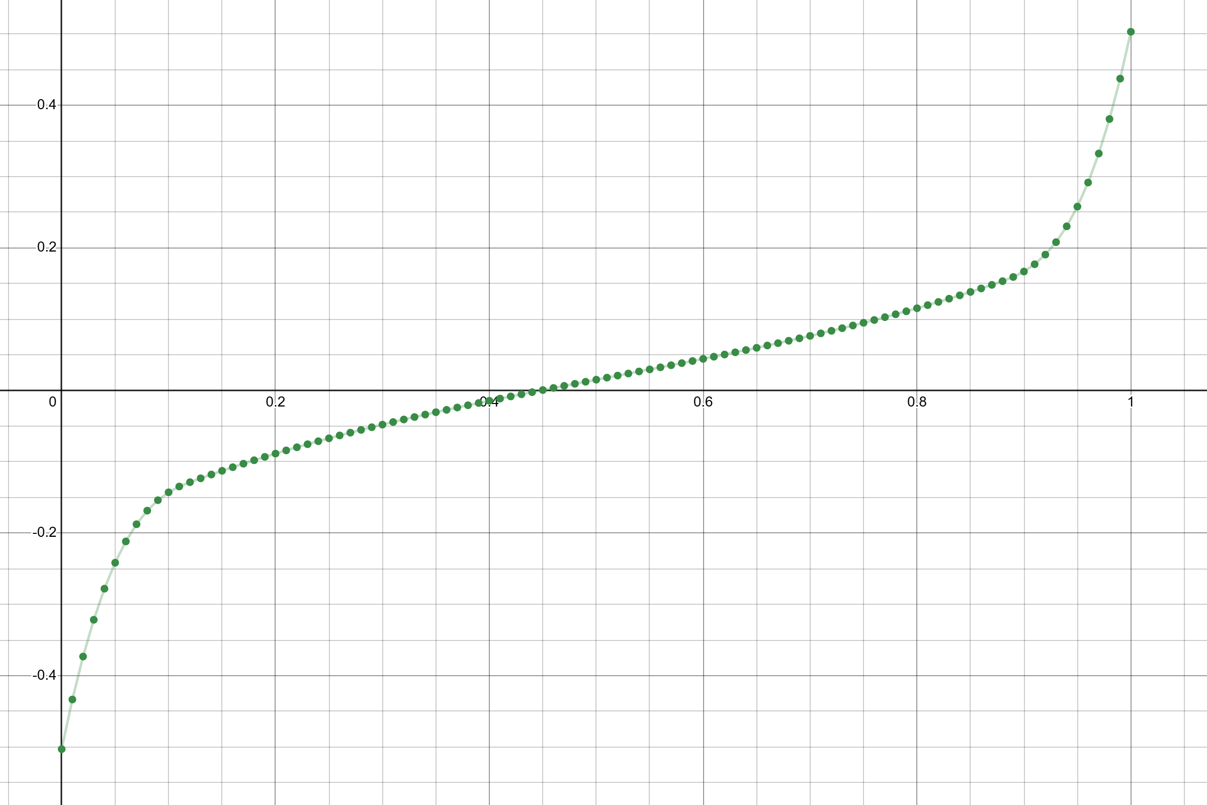Lethal Company’s randomiser curve sampled at 101 points.

Approximating using Least-Squares Regression

Initially, I noticed that the curve could be approximated by a function of the form

$$mx+a\arctan (b\tan (cx+d)+k),$$

where $m$, $a$, $b$, $c$, $d$, and $k$ are constants and the domain of $x$ is $[0,1]$. If the values for the constants in the following table are used, then the approximation is quite good, with an $r^2$ value of $0.999$⁶.

Constant	Approximate Value
$a$	−0.326786244784
$b$	0.115164070585
$c$	−3.08270565794
$d$	1.57079632679
$k$	0.209865018049
$m$	0.165967731215

The explicit formula given by these coefficients is approximately

$$R(x)\approx 0.1659677x-0.3267862\arctan (0.1151641\tan (1.570796-3.082706x)+0.2098650).$$

The Lethal Company Wiki states that the randomiser curve can be approximated using the function

$$\frac{1}{16.6063}\ln \left(\frac{x}{1-x}\right).$$

While this function does approximate the shape of the original curve, it diverges more from its shape than our initial approximation, as visible in the following comparison. Note that the original curve is coloured green, the Wiki’s approximation in blue, and the arctangent approximation in red.

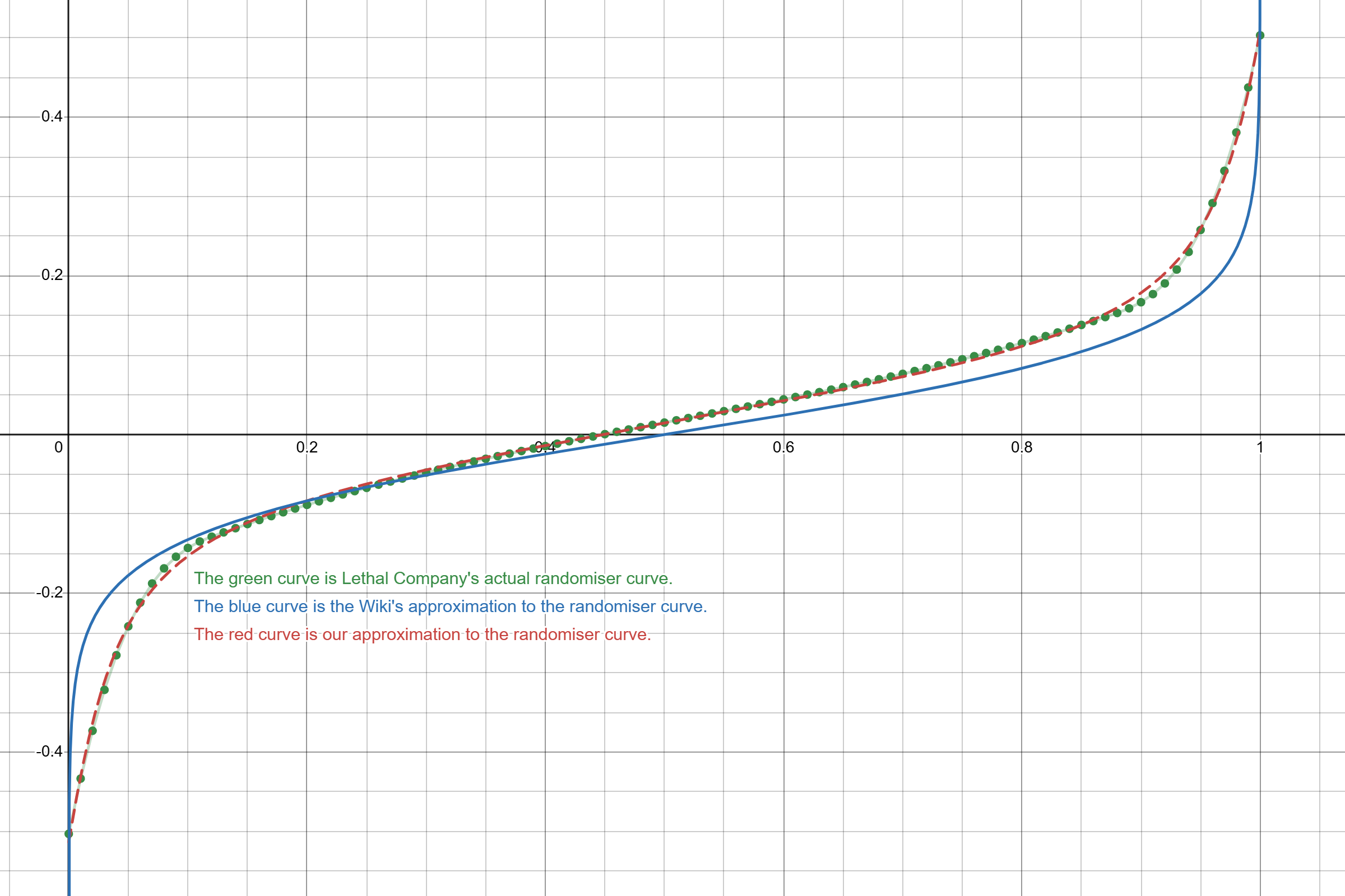Comparison between Lethal Company’s Randomiser Curve, a Logarithmic approximation, and an Arctangent approximation.

Nevertheless, the simplicity of the wiki’s formula offers a less precise but easier to calculate formula for approximating the randomiser curve.

I’ve set up a Desmos plot where you can play around with this curve. Feel free to play around with the shape of the approximation function!

Explicit Formula using Non-Linear Interpolation

We can do better!

Thanks to my sister Seukari for helping with this part of the post! 🙂 (She’s so smart and knows all about Unity.)

In short, our problem with the randomiser curve is that we have a set of points we can sample but we don’t know the exact shape of the curve. One of the ways we can try finding the shape of the original curve from a set of points is through something called interpolation. In short, interpolation is a way of finding a curve which fits (or more-or-less fits) a set of discrete data points, which is exactly what we want to do! One way to do this is using spline interpolation, where the set of points is approximated by piecewise polynomials, that is, a bunch of polynomials defined for each piece of the curve, which all fit together smoothly to form the entire function. One of the most common methods of spline interpolation is through Bézier curves, which you might’ve heard of.

However, it turns out the randomiser curve is defined using Cubic Hermite splines, and we can figure out that the exact (barring floating-point precision errors) shape of the randomiser curve is given by:

$$R(x)=\{\begin{array}{ll}120.0178x^3-50.53573x^2+7.455404x-0.5030289& \text{ if }0\le x\le 0.117235\\ 0.5730645x^3-0.8789711x^2+0.7373449x-0.2054627& \text{ if }0.117235<x\le 0.8803625\\ 120.8263x^3-313.5079x^2+271.5885x-78.40379& \text{ if }0.8803625<x\le 1\\ 0& \text{ otherwise}\end{array}$$

The following comparison shows that this approximation perfectly describes the shape of the randomiser curve observed from the sampled points.

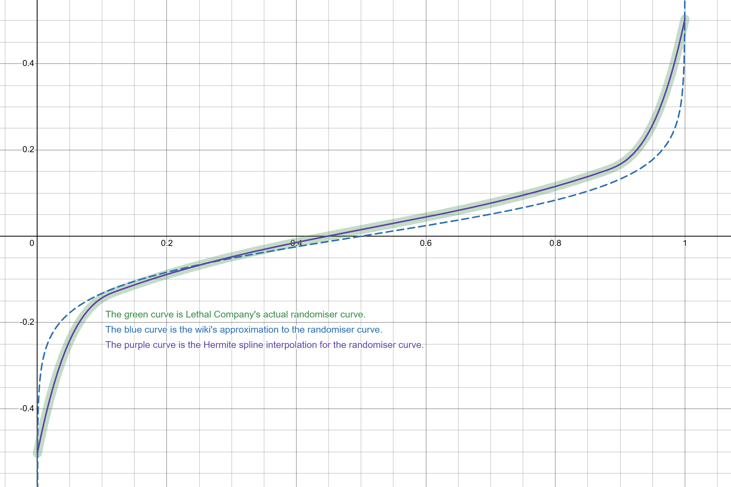Comparison between Lethal Company’s Randomiser Curve, a Logarithmic approximation, and a Hermite spline interpolation.

This is the exact curve that Unity uses (the coefficients of this formula were computed within Unity itself) to evaluate the randomiser curve at an arbitrary point.

You can play around with this function using this Desmos plot. Additionally, feel free to use the following Mathematica code, which I used to compute the function!

(* AnimationCurve Keyframe Data *)
X = {0, 0.117235, 0.8803625, 1};
Y = {-0.5030289, -0.1301773, 0.1534421, 0.5030365};
Tangents = {7.455404, 0.5548811, 0.5221589, 7.051469};

(* Auxiliary Functions *)
a[k_] := ((X[[k + 1]] - X[[k]])*(Tangents[[k + 1]] + Tangents[[k]]) - 2*(Y[[k + 1]] - Y[[k]])) /
    (X[[k + 1]] - X[[k]])^3

b[k_] := (3 *(Y[[k + 1]] - Y[[k]]) - (X[[k + 1]] - X[[k]]) * 
    (Tangents[[k + 1]] + 2*Tangents[[k]]))/(X[[k + 1]] - X[[k]])^2

(* Coefficient of each Term in the Hermite Spline *)
CoefficientXCubed[k_] := a[k]
CoefficientXSquared[k_] := b[k] - 3*X[[k]]*a[k]
CoefficientX[k_] := Tangents[[k]] - X[[k]]*(b[k] + CoefficientXSquared[k])
FreeCoefficient[k_] := (X[[k]]^2)*(b[k] - a[k]*X[[k]]) - Tangents[[k]]*X[[k]] + Y[[k]]

(* Function Definition *)
R[k_, x_] := CoefficientXCubed[k]*(x^3) + CoefficientXSquared[k]*(x^2) + 
  CoefficientX[k]*x + FreeCoefficient[k]

RandomiserCurve[x_] := Piecewise[{
   {R[1, x], X[[1]] <= x <= X[[2]]},
   {R[2, x], X[[2]] < x <= X[[3]]},
   {R[3, x], X[[3]] < x <= X[[4]]}  
}]

Explicit Formula for the $n$-th Quota

Equation $\text{(3)}$ gives what is known as a recurrence relation describing the sequence of quotas $Q_n$.

Turns out this recurrence is somewhat straightforward to solve to obtain a direct, explicit formula for the $n$-th quota. Let’s start by applying the recurrence relation and seeing if we can notice a pattern:

1. $Q_1=130$
2. $Q_2\approx Q_1+B(1+s\cdot 1^2)(1+mR({\ell }^{\ast }{U}_1))$
3. $Q_3\approx Q_1+B(1+s\cdot 1^2)(1+mR({\ell }^{\ast }{U}_1))+B(1+s\cdot 2^2)(1+mR({\ell }^{\ast }{U}_2))$
4. …

All we did was replace $Q_2$ in the formula for $Q_3$, but hopefully you should already see a pattern starting to emerge! It looks like we take $Q_1$, the starting quota, then add a term for $n=1$, then the same term but with $n=2$, and so on. We won’t concern ourselves with proving that this is always correct⁷, and we thus just assume that the $n$-th quota is given by

$$\begin{array}{}\text{(5)}& Q_n\approx Q_1+B\sum _{k=1}^{n-1}(1+s{k}^2)(1+mR({\ell }^{\ast }{U}_k)).\end{array}$$

For the less mathematically-inclined but tech-savvy readers out there, that large scary symbol is just a for loop, and it’s known as the summation operator.

This general formula allows us to calculate the minimum and maximum possible values for each quota. Note that, since $R(x)$ is a strictly increasing function in $[0,1]$, it attains a global minimum $R(0)$ at $x=0$ and a global maximum $R(1)$ at $x=1$. Thus, $Q_n$ attains a global minimum when each $U_k$ in the sum evaluates to 0, and a global maximum when each $U_k$ in the sum evaluates to 1. Define the function

$$Q_n(u)=Q_1+B\sum _{k=1}^{n-1}(1+s{k}^2)(1+mR({\ell }^{\ast }u))=Q_1+\frac{B(1+mR({\ell }^{\ast }u))}{6}(n-1)(2s{n}^2-sn+6),$$

where $u$ is any real number in $[0,1]$. Then, we have

$$Q_n(0)\le Q_n\le Q_n(1).$$

Since each quota is an integer value, we can write

$$\begin{array}{}\text{(6)}& \lceil Q_n(0)\rceil \le Q_n\le \lfloor Q_n(1)\rfloor ,\end{array}$$

where $\lceil \cdot \rceil$ and $\lfloor \cdot \rfloor$ denote the floor and ceiling functions, respectively.

Probability Distribution of the $n$-th Quota

Equation $\text{(5)}$ describes the random variable $Q_n$ and we could thus obtain a function, known as a Probability Density Function (PDF), describing the probability of $Q_n$ taking each possible number value. However, note that since each $R({\ell }^{\ast }{U}_k)$ term in the sum is itself a random variable, we’re dealing with an arbitrary sum of random variables, and doing algebra with random variables really complicates things. You could even say it gets convoluted - literally.

What we can do instead is use Equation $\text{(3)}$ to derive a recurrence relation for the probability density functions of each $Q_n$. Let’s start by setting

$$X_n=B(1+s{n}^2)(1+mR({\ell }^{\ast }{U}_n))$$

so that Equation $\text{(5)}$ becomes $Qn+1=Q_n+X_n$. From this equation, we know that the PDF of $Q_{n+1}$ is given by the convolution between the PDFs of $Q_n$ and $X_n$,

$$f_{Q_{n+1}}(q)\approx {\int }_{-\mathrm{\infty }}^{+\mathrm{\infty }}{f}_{Q_n}(t)f_{X_n}(q-t)dt,$$

where we use $f_X$ to denote the PDF of a random variable $X$. Then, we just need to find the PDF of $X_n$! Thankfully, this is easy to do:

$$f_{X_n}(x)=\frac{d}{dx}{F}_x(x)=\frac{d}{dx}Pr(X_n\le x),$$

where $F_X$ is the Cumulative Distribution Function (CDF) of $X$. This is easy to achieve from the definition of $X_n$, yielding

$$F_{X_n}(x)\approx Pr(X_n\le x)=Pr(U_n\le \frac{1}{{\ell }^{\ast }}{R}^{-1}(\frac{x}{mB(1+s{n}^2)}-\frac{1}{m})).$$

Since $U_n$ follows a continuous uniform distribution, we immediately get

$$F_{X_n}(x)\approx \frac{1}{{\ell }^{\ast }}{R}^{-1}(\frac{x}{mB(1+s{n}^2)}-\frac{1}{m}),$$

which gives

$$f_{X_n}(x)\approx \frac{a_n}{{\ell }^{\ast }{R}^{\prime }(R^{-1}(a_{n}x-b))},$$

where $a_n=1/(mB(1+s{n}^2))$ and $b=1/m$.

This finally allows us to express our recurrence relation for the PDF of $Q_n$, which becomes

$$\begin{array}{}\text{(7)}& f_{Q_{n+1}}(q)\approx \frac{a_n}{{\ell }^{\ast }}{\int }_{-\mathrm{\infty }}^{+\mathrm{\infty }}\frac{f_{Q_n}(t)}{R^{\prime }(R^{-1}(a_n(q-t)-b))}dt.\end{array}$$

The base case is $f_{Q_1}(q)=\delta (q-Q_1)=\delta (q-130)$, where $\delta (x)$ denotes the Dirac delta function, since the first quota, $Q_1$, is always a fixed value. If you want to be really rigorous, you could say $Q_1$ is a random variable following a degenerate distribution with parameter $k_0=130$.

While it would be intractable to express a general formula for $f_{Q_n}(q)$⁸, we can at least obtain the conditional CDF of a quota if we know the value of the previous quota. This is given by

$$Pr(Q_{n+1}\le q\mid Q_n=p)=Pr(p+X_n\le q)=Pr(X_n\le q-p)=F_{X_n}(q-p),$$

which gives

$$Pr(Q_{n+1}\le q\mid Q_n=p)\approx \frac{1}{{\ell }^{\ast }}{R}^{-1}(\frac{q-p}{mB(1+s{n}^2)}-\frac{1}{m}).$$

Calculating the Average Quota

Since we have obtained a general formula for $Q_n$, the $n$-th quota, we can simply denote its average value as $\text{E}[Q_n]$ and use the formula in Equation $\text{(5)}$, obtaining

$$\text{E}[Q_n]\approx \text{E}[Q_1+B\sum _{k=1}^{n-1}(1+s{k}^2)(1+mR({\ell }^{\ast }{U}_k))].$$

How on Earth do we calculate anything with this monstrosity? Well, remember how I said the expected value operator was linear? Recall that, if we have two random variables $X$ and $Y$ and two numbers $a$ and $b$, then $\text{E}[aX+bY]=a\text{E}[X]+b\text{E}[Y]$. This lets us simplify the above equation to the simpler form

$$\text{E}[Q_n]\approx Q_1+B\sum _{k=1}^{n-1}(1+s{k}^2)(1+m\text{E}[R({\ell }^{\ast }{U}_k)])$$

where, since every $U_k$ (for all $k$) is identically distributed, we can factor out the $(1+m\text{E}[R({\ell }^{\ast }{U}_k)])$ to obtain

$$\text{E}[Q_n]\approx Q_1+B(1+m\text{E}[R({\ell }^{\ast }U)])\sum _{k=1}^{n-1}(1+s{k}^2).$$

Finally, it turns out that the sum gives rise to an explicit formula⁹, allowing us to write

$$\text{E}[Q_n]\approx Q_1+\frac{1}{6}B(1+m\text{E}[R({\ell }^{\ast }U)])(n-1)(2s{n}^2-sn+6).$$

Almost there! We’re so close to an explicit formula for the average $n$-th profit quota. All we’re missing is a way to get rid of the $\text{E}[R({\ell }^{\ast }U)]$ term, which we haven’t calculated yet. Thankfully, this is somewhat straightforward using the law of the unconscious statistician:

$$\text{E}[R({\ell }^{\ast }U)]={\int }_{-\mathrm{\infty }}^{+\mathrm{\infty }}R({\ell }^{\ast }x)f_U(x)dx={\int }_0^{1}R({\ell }^{\ast }x)dx=\frac{1}{{\ell }^{\ast }}{\int }_0^{{\ell }^{\ast }}R(x)dx.$$

And that’s it! We have a general formula for approximating the $n$-th profit quota in Lethal Company:

$$\text{E}[Q_n]\approx Q_1+\frac{1}{6}B(1+m{\int }_0^{1}R({\ell }^{\ast }x)dx)(n-1)(2s{n}^2-sn+6),$$

or, by using the known values for the coefficients,

$$\begin{array}{}\text{(8)}& \text{E}[Q_n]\approx 130+\kappa (n-1)(\frac{n^2}{8}-\frac{n}{16}+6),\end{array}$$

where $\kappa$ is given by

$$\kappa =\frac{100}{6}(1+\frac{1}{{\ell }^{\ast }}{\int }_0^{{\ell }^{\ast }}R(x)dx).$$

Calculating the Quota Variance

We already have an explicit formula for the average quota, but… how do we know how close the quota will actually be to this value? Can we calculate the standard deviation?

Yes! Let’s do it. We can start by using Equation $\text{(3)}$ to write

$$\text{Var}(Q_{n+1})\approx \text{Var}(Q_n+B(1+s{n}^2)(1+mR({\ell }^{\ast }{U}_n))).$$

Now, while $Q_{n+1}$ depends on the random value taken by $U_n$, the previous quota $Q_n$ does not depend on $U_n$, and we can thus say the two are independent. Then, using the properties for the variance operator we saw at the beginning of the post, we can simplify this formula to

$$\begin{array}{}\text{(9)}& \text{Var}(Q_{n+1})\approx \text{Var}(Q_n)+(mB(1+s{n}^2){)}^2\text{Var}(R({\ell }^{\ast }{U}_n)).\end{array}$$

Since $\text{Var}(X)=\text{E}[X^2]-\text{E}[X{]}^2$, we can calculate the variance of $R(U_n)$ to be

$$\text{Var}(R(U_n))=\text{E}[R^2({\ell }^{\ast }{U}_n)]-\text{E}[R({\ell }^{\ast }{U}_n){]}^2.$$

We already have a formula for $\text{E}[R(U_n)]$, and $\text{E}[R^2(U_n)]$ can once again be expressed using the law of the unconscious statistician:

$$\text{E}[R^2(U_n)]={\int }_0^1{R}^2({\ell }^{\ast }x)dx=\frac{1}{{\ell }^{\ast }}{\int }_0^{{\ell }^{\ast }}{R}^2(x)dx.$$

We can then solve the recurrence in Equation $\text{(9)}$ very similarly to how we solved Equation $\text{(3)}$, yielding the general formula

$$\text{Var}(Q_n)\approx \frac{m^2{B}^2(\text{E}[R^2(U)]-\text{E}[R(U){]}^2)}{30}(n-1)(6s^2{n}^4-9s^2{n}^3+s(s+20)n^2+s(s-10)n+30),$$

or, once again using the known values for the coefficients,

$$\begin{array}{}\text{(10)}& \text{Var}(Q_n)\approx K(n-1)(\frac{3n^4}{128}-\frac{9n^3}{256}+\frac{321n^2}{256}-\frac{159n}{256}+30),\end{array}$$

where $K$ is given by

$$K=\frac{1000}{3{\ell }^{\ast }}({\int }_0^{{\ell }^{\ast }}{R}^2(x)dx-\frac{1}{{\ell }^{\ast }}{({\int }_0^{{\ell }^{\ast }}R(x)dx)}^2).$$

I’ve set up a Desmos plot where you can play around with the formulae for the average quota and the variance.

Total Scrap Required and Average Per Day

There are two more formulas which we can easily obtain from the expected quota value. Let $T_n$ denote the total amount of scrap value needed to meet the $n$-th quota, and $D_n$ the scrap value needed to collect per day to meet the $n$-th quota. Then, we have

$$T_n=\sum _{k=1}^n{Q}_k$$

and

$$D_n=\frac{T_n}{3n}=\frac{1}{3n}\sum _{k=1}^n{Q}_k.$$

Intuitively, the total scrap value needed to complete any quota is that quota along with the sum of all previous quotas, and we can divide this value by the number of days from the beginning of the game (3 days per quota) to get the daily scrap value needed.

The expected value for these quantities is given directly by the expected value of $T_n$,

$$\text{E}[T_n]=Q_1+\sum _{k=2}^n\text{E}[Q_k]\approx n{Q}_1+\frac{B(1+m\text{E}[R(U)])}{6}\sum _{k=2}^n(k-1)(2s{k}^2-sk+6),$$

where the sum can itself be evaluated to give the general closed formula

$$\text{E}[T_n]\approx n{Q}_1+\frac{B(1+m\text{E}[R(U)])}{12}(s{n}^4+(6-s)n^2-6n).$$

From this, we easily obtain

$$\text{E}[D_n]\approx \frac{Q_1}{3}+\frac{B(1+m\text{E}[R(U)])}{36}(s{n}^3+(6-s)n-6).$$

The variance (and therefore the standard deviation) of these variables cannot be easily calculated as for the $n$-th quota, as they are formed by sums of dependent random variables. We’ll just have to make do with the average value.

Finally, using the explicit values for the coefficients we can write

$$\begin{array}{}\text{(11)}& \text{E}[T_n]\approx 130n+\frac{\kappa }{2}(\frac{n^4}{16}+\frac{95n^2}{16}+6n)\end{array}$$

and

$$\begin{array}{}\text{(12)}& \text{E}[D_n]\approx \frac{130}{3}+\frac{\kappa }{6}(\frac{n^3}{16}+\frac{95n}{16}-6),\end{array}$$

where $\kappa$ is defined as in Equation $\text{(8)}$.

General Results

General Formulae

The average value of the $n$-th profit quota can be approximated by

$$\text{E}[Q_n]\approx 130+\kappa (n-1)(\frac{n^2}{8}-\frac{n}{16}+6).$$

The variance of the $n$-th profit quota can be approximated by

$$\text{Var}(Q_n)\approx K(n-1)(\frac{3n^4}{128}-\frac{9n^3}{256}+\frac{321n^2}{256}-\frac{159n}{256}+30).$$

The average total scrap value required to complete the $n$-th quota can be approximated by

$$\text{E}[T_n]\approx 130n+\frac{\kappa }{2}(\frac{n^4}{16}+\frac{95n^2}{16}+6n).$$

The average daily scrap value required to complete all quotas up to the $n$-th quota can be approximated by

$$\text{E}[D_n]\approx \frac{130}{3}+\frac{\kappa }{6}(\frac{n^3}{16}+\frac{95n}{16}-6).$$

For all these formulae, $\kappa$ and $K$ are terms given by

$$\kappa =\frac{100}{6}(1+\frac{1}{{\ell }^{\ast }}{\int }_0^{{\ell }^{\ast }}R(x)dx)$$

and

$$K=\frac{1000}{3{\ell }^{\ast }}({\int }_0^{{\ell }^{\ast }}{R}^2(x)dx-\frac{1}{{\ell }^{\ast }}{({\int }_0^{{\ell }^{\ast }}R(x)dx)}^2),$$

where $R$ denotes Lethal Company’s quota randomiser curve and ${\ell }^{\ast }=|\ell -1|$, where $\ell$ is the player’s luck value.

The minimum and maximum values of the $n$-th profit quota are respectively given by

$$min{Q}_n\approx \lceil 130+8.28285166667(n-1)(\frac{n^2}{8}-\frac{n}{16}+6)\rceil$$

and

$$max{Q}_n\approx \lfloor 130+25.0506083333(n-1)(\frac{n^2}{8}-\frac{n}{16}+6)\rfloor ,$$

where $\lceil \cdot \rceil$ and $\lfloor \cdot \rfloor$ denote the floor and ceiling functions, respectively.

Quota Tables

The following tables, much like the one in the Lethal Company Wiki, present the average quota values, along with the total scrap value required to collect and how that translates to the average scrap value collected per day. The average scrap per day is how much scrap value you need to collect per day, on average, to meet that quota, taken over the duration of the run! That is, if you wished to meet quota 10, you should collect an average of 369 scrap value per day since the beginning of your run.¹⁰

We now present these tables with values related to the first $25$ quotas for three different luck values.

Neutral Luck ($\ell =0$)

If the player’s luck remains at $0$, then the quota system functions identically to the pre-v65 system!

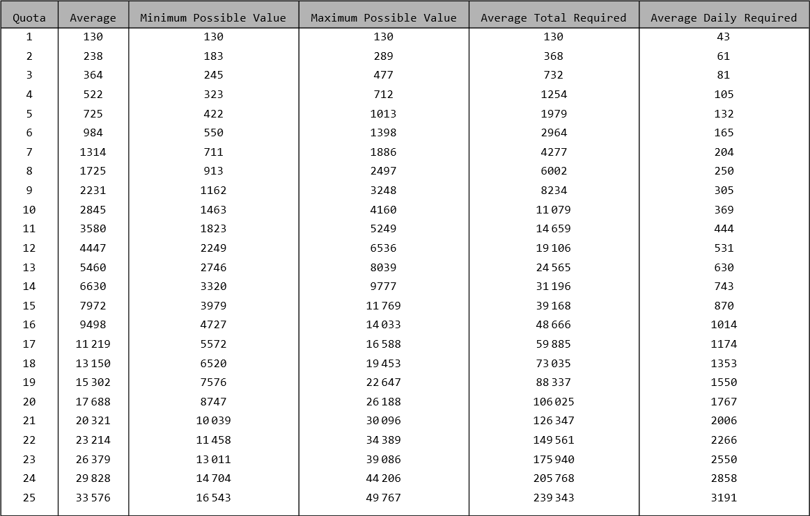First 25 Lethal Company quotas, for a luck value of 0.

Worst Luck ($\ell =-0.012$)

I actually don’t know why these values actually ended up being slightly lower than those for $\ell =0$… maybe negative luck just isn’t that different from neutral luck?

First 25 Lethal Company quotas, for the lowest possible luck value.

Best Luck ($\ell =0.1545$)

First 25 Lethal Company quotas, for the highest possible luck value.

If you’re curious, I generated the values to fill these tables using the following Mathematica code. Feel free to use it if you want!

m = 1; (* Randomiser Multiplier *)
s = 1/16; (* Increase Steepness *)
B = 100; (* Base Increase*)

Q1 = 130; (* Starting Quota *)

PlayerLuck = 0.1545;  (* Luck is between -0.012 and 0.1545 *)
LuckMultiplier = Abs[PlayerLuck - 1];

(* Probability Distribution of the n-th Quota *)
Quota[1] = ProbabilityDistribution[DiracDelta[x - Q1], {x, -Infinity, +Infinity}];
Quota[n_] := Quota[n] = 
   TransformedDistribution[
    q + B*(1 + s*(n - 1)^2)*(1 + m*RandomiserCurve[LuckMultiplier*u]), 
    {q \[Distributed] Quota[n - 1], u \[Distributed] UniformDistribution[]}
];

AvgQuota[n_] := AvgQuota[n] = NExpectation[x, x \[Distributed] Quota[n]];
VarQuota[n_] := VarQuota[n] = Variance[Quota[n]];
StdevQuota[n_] := StdevQuota[n] = StandardDeviation[Quota[n]];
AvgTotalRequired[n_] := AvgTotalRequired[n] = Sum[AvgQuota[k], {k, 1, n}];
AvgDailyRequired[n_] := AvgDailyRequired[n] = AvgTotalRequired[n]/(3 n);

(* Minimum value (u = 0) and maximum value (u = 1) for the n-th Quota *)
QuotaBound[n_, u_] := Q1 + B*(1 + m*RandomiserCurve[LuckMultiplier*u])*(n - 1)*(2*s*n^2 - s*n + 6)/6;
QuotaLowerBound[n_] := Ceiling[QuotaBound[n, 0]];
QuotaUpperBound[n_] := Floor[QuotaBound[n, 1]];

NumQuotas = 25;
AveragesTable = 
  Table[Round /@ {i, AvgQuota[i], QuotaLowerBound[i], 
     QuotaUpperBound[i], AvgTotalRequired[i], 
     AvgDailyRequired[i]}, {i, NumQuotas}
    ];
Grid[
  Prepend[
   AveragesTable, {"Quota", "Average", "Minimum Possible Value", 
    "Maximum Possible Value", "Average Total Required", 
    "Average Daily Required"}],
  Frame -> All
];
Insert[%, {Background -> {None, {GrayLevel[0.7], {White}}}, 
  Dividers -> {Black, {2 -> Black}}, Frame -> True, 
  Spacings -> {2, {2, {0.7}, 2}}}, 2
]
Export["QuotaTable_Luck"<>ToString[PlayerLuck]<>".png", %]

Luck Values

The following table presents the luck value the player gains by acquiring each unlockable item for their ship.

Decorative Item	Luck Value
Orange Suit	0
Green Suit	0
Hazard Suit	0
Pajama Suit	0
Cozy Lights	0.005
Teleporter	0
Television	0.02
Cupboard	0
File Cabinet	0
Toilet	0.01
Shower	0.015
Light Switch	0
Record Player	0.005
Table	0.004
Romantic Table	0.005
Bunkbeds	0
Terminal	0
Signal Translator	-0.012
Loud Horn	0.0025
Inverse Teleporter	0.004
Jack-O-Lantern	0.012
Welcome Mat	0.003
Goldfish	0.006
Plushie Pajama Man	0.003
Purple Suit	0
Bee Suit	0
Bunny Suit	0
Disco Ball	0.06

Consequences for Moon-Exclusive High Quota Runs

Using the above results, we can establish some limits on how long a moon-exclusive high quota speedrun can be viable!

Thanks to Sikorski, a fellow member of the Sheff’s Kitchen server on Discord, for helping with these sections! 🙂

The game’s code that needed to be analysed for the following analysis mainly consists of the RoundManager.SpawnScrapInLevel, RoundManager.GetRandomWeightedIndex, and TimeOfDay.SetNewProfitQuota methods. The relevant logic was re-implemented in Python to enable the required custom analysis. The used code spans several files and several hundred lines, and is thus not presented in this article.

Daily Scrap Value per Moon

In the following sections, we cover the amount of scrap value spawned per day on each moon. We additionally argue for a computational approach, as opposed to the analytical approach we have taken so far, due to the prohibitive difficulty of mathematically modelling Lethal Company’s scrap spawning behaviour.

In short, instead of analytically calculating the PDFs related to scrap spawn, we run a large number of simulations so as to sample a large number of values from the probability distribution we wish to describe. Then, we apply Kernel Density Estimation (KDE), which approximates the “true” PDF using other functions, known in this context as kernels. Mathematically, the PDF $f_X(x)$ of a random variable $X$ can be approximated using

$$f_X(x)\approx \frac{1}{Nh}\sum _{i=1}^{N}K\left(\frac{x-x_i}{h}\right),$$

where $x_i$ denotes the $i$-th sample, $N$ is the total number of samples, and $h$ is an arbitrary smoothing parameter usually called the bandwidth of the estimator.

In our calculations, we use the gaussian_kde method provided by the SciPy Python library, which provides an easy-to-use API for calculating the KDE given a set of samples. Specifically, it uses Gaussian kernels, i.e. $K(x)=\varphi (x)$, where $\varphi$ denotes the PDF of a Standard normal distribution.

Interior Scrap

In order to properly simulate scrap spawns, we have to take a few things into account. Firstly, each moon has a uniformly random varying total amount of scrap that it spawns between predefined minimum and maximum bounds. In addition to this, each moon has a set of possible items that can spawn with their respective probabilities. Finally, each item itself has a uniformly random value generated between its minimum and maximum scrap values.

Mathematically, the total scrap value $L$ (which is a random variable) can be written,

$$L=\sum _{i=1}^N{U}_i(S),$$

where $S$ is the scrap type, $U_i$ is the individual scrap value, which depends on the scrap type chosen, and $N$ is the total number of scrap, with all of these values constituting random variables. What makes it difficult to proceed analytically is:

1. The depedency of $U_i$ on $S$. We can think of $U_i$ as being a uniform pdf, yet it changes depending on what type of scrap is selected. This, by itself, is not completely impossible to work around, as in principle one could consider a huge piece-wise function where $S$ is simply a random number whose value determines from which uniform PDF we are drawing from. However…
2. The dependency of the upper-bound on the sum is what makes us an analytic approach markedly intractable. Unfortunately, we cannot even expand the sum simply because we do not know if the terms will exist or not.

Furthermore, the following needs to be considered:

1. The Factory interior type always guarantees an Apparatus spawn, which is worth a fixed 80 scrap value;
2. The Mineshaft interior type guarantees the spawn of an extra 6 scrap items.

Finally, we need to consider the possibility of single scrap events, in which all generated scrap on a moon for the day is replaced with a single type of scrap. The probability that this happens is based on the chosen item’s rarity, and individual scrap value is adjusted based on the total generated scrap value. This further serves to support the argument of a computational (as opposed to an analytical) approach, as the individual scrap value is now dependent upon total scrap value. The following, taken directly from the game’s code, handles the logic for determining whether a single scrap event will occur. In particular, if num3 != -1, then num3 represents the scrap item which will be used for the event.

int num3 = -1;
if (this.AnomalyRandom.Next(0, 500) <= 25)
{
	num3 = this.AnomalyRandom.Next(0, this.currentLevel.spawnableScrap.Count);
	bool flag = false;
	for (int n = 0; n < 2; n++)
	{
		if (this.currentLevel.spawnableScrap[num3].rarity >= 5 && !this.currentLevel.spawnableScrap[num3].spawnableItem.twoHanded)
		{
			flag = true;
			break;
		}
		num3 = this.AnomalyRandom.Next(0, this.currentLevel.spawnableScrap.Count);
	}
	if (!flag && this.AnomalyRandom.Next(0, 100) < 60)
		num3 = -1;
}

The following flowchart illustrates this logic in a more readable format. Note that this logic is only executed with a $26/500=5.2\mathrm{\%}$ chance.

Logic for determining if a single scrap event executes.

Beehives and Entities

We now address the possible scrap value that can be gained from entity spawns, e.g. Butler knives and Nutcracker shotguns/shells, and why we consider hives and not these other sources of scrap. The simple answer is just that taking into account the enemy spawns is just too complicated. In this project, we assume that player skill is not a factor; the employees will play with 100% efficiency and their skills will not play a role in the amount of scrap that can be gained.

The way in which entities are determined to spawn is a complicated process that is neatly detailed on this LC wiki page. The main point is that whether or not an entity spawns depends on:

1. The number of entities of that type has already spawned (either through the maximum number spawned or the fact that a type of entity is more likely to spawn if other entities of that type have already spawned);
2. The number of total entities that have spawned (through the indoor/outdoor/daytime power levels).

The point is that entity spawns are strictly not independent events. This makes including the Butler knives, shotguns, and shells into the scrap value PDF prohibitively difficult.

This is all opposed to beehives which, in the case of both conditions, only ever spawn at the beginning of the day, and are therefore not subjected to the dependence on other entity spawns. Up to 6 hives can spawn with a fixed probability on every moon. For example, on Experimentation, since there is a $14.86\mathrm{\%}$ chance to spawn a hive, then there is a $(14.86\mathrm{\%}{)}^2=2.21\mathrm{\%}$ to spawn two hives, $(14.86\mathrm{\%}{)}^3=0.33\mathrm{\%}$ to spawn three, and so on. In general, the probability of $n$ beehives spawning is given by $p^n$, where $p$ is the probability of spawning a hive on a given moon, which is easy to calculate directly.

In terms of value, beehives can be worth as anywhere from 40 to 150 scrap value (compared with a fixed 35, 60, and 30 for knife, shotgun, and shotgun shells, respectively). Thus, we consider beehives capable of influencing the pace of a run, and therefore count them towards the total scrap value on a moon in our calculations.

Total Scrap Value

Using the previous logic, we re-implement the game’s RoundManager.SpawnScrapInLevel function, which handles (as the name implies) spawning interior scrap when the player enters a moon. Then, coupled with the logic for simulating beehive spawns, we run $N={10}^7$ simulations and apply Kernel Density Estimation, as described above, to estimate the distribution of the total scrap value that can be spawned each day on each moon.

In order to perform these calculations, the game’s code had to be analysed to obtain the spawn chances of beehives and each scrap item on each moon, along with the chance of each interior being used. Curiously, these values are presented in the game’s code for the moon 44 Liquidation, even though it is not currently implemented. For curiosity’s sake, we thus include it in our analysis.

These distributions are illustrated in the following figure.

Distributions of daily scrap value spawned on each moon.

Limits on High-Quota Runs

The following sections assume the following: the player is using a mod which removes the cost of travelling to paid moons; gift boxes are sold as-is, without being opened. These assumptions are required to enable calculations to be performed.

In Lethal Company, you only meet a profit quota if you manage to sell a total scrap value greater than or equal to that quota. This doesn’t necessarily mean you need to find that amount of scrap value on moons in the 3 days of a quota’s duration, as you can accumulate scrap from previous runs on the ship if you don’t oversell.

Let ${\text{Acc}}_n$ be the total amount of scrap value you have accumulated on the ship at the end of the $n$-th quota. Then,

$${\text{Acc}}_n=\sum _{k=1}^{3n}{L}_k-\sum _{k=1}^n{Q}_k,$$

where $L_k$ denotes the daily scrap value spawned on an arbitrary moon on the $k$-th day of the entire run. We can simplify this formula to

$${\text{Acc}}_n={\mathcal{L}}_n-T_n,$$

where ${\mathcal{L}}_n=\sum _{k=1}^{3n}{L}_k$ and $T_n$ denotes the total scrap value needed to meet the $n$-th quota.

To successfuly meet the $n$-th quota, we thus need to have enough accumulated scrap value from the previous run which, along with whatever we can loot in 3 days, is greater than or equal to the objective quota. Mathematically,

$${\text{Acc}}_{n-1}+L_{3n-2}+L_{3n-1}+L_{3n}\ge Q_n⟺{\text{Acc}}_{n-1}+(L_{3n-2}+L_{3n-1}+L_{3n}-Q_n)\ge 0⟺{\text{Acc}}_n\ge 0,$$

where we take the ordering $X\ge Y$ between two random variables $X$ and $Y$ to denote the deterministic dominance of $X$ over $Y$.

We thus have the condition ${\text{Acc}}_n\ge 0$ for meeting the $n$-th quota. Using the defintion of ${\text{Acc}}_n$, we can write

$${\mathcal{L}}_n-T_n\ge 0,$$

which can be simplified to yield ${\mathcal{L}}_n\ge T_n$.

Intuitively, the total generated scrap value throughout the entirety of a run must be enough to meet the sum total of each quota in the run. A run thus becomes impossible if ${\mathcal{L}}_n<T_n$.

Thus, there exists a hard limit for single-moon high quota runs, with the highest achievable quota being the $n$-th quota, where $n$ is the largest integer such that

$${\mathcal{L}}_n\ge T_n,$$

or, equivalently, using the definition of deterministic dominance,

$$Pr({\mathcal{L}}_n\ge T_n)=1⟺Pr({\mathcal{L}}_n<T_n)=0.$$

An explicit definition of this value of $n$ is given by

$$n=max\{k\in \mathbb{N}:Pr({\mathcal{L}}_k<T_k)=0\},$$

which can be expanded to

$$n=max\{k\in \mathbb{N}:{\int }_{-\mathrm{\infty }}^{-\mathrm{\infty }}(f_{T_k}(x){\int }_{-\mathrm{\infty }}^x{f}_{{\mathcal{L}}_k}(y)dy)dx=0\}.$$

We thus obtain the PDFs $f_{{\mathcal{L}}_k}(y)$ and $f_{T_k}(x)$ using Kernel Density Estimation on $N={10}^4$ samples¹¹, as previously described, and then calculate the integral using the resulting functions. If we do so for increasing values of $k$, we can get the probability of each quota not being possible. Alternatively, we can calculate $1-Pr({\mathcal{L}}_k<T_k)$ to know the probability of the $k$-th quota being possible. The results of these calculations are illustrated in the following figures.

Neutral Luck ($\ell =0$)

Probability of not enough scrap spawning to complete the quota, for a luck value of 0.

Worst Luck ($\ell =-0.012$)

Probability of not enough scrap spawning to complete the quota, for the lowest possible luck value.

Best Luck ($\ell =0.1545$)

Probability of not enough scrap spawning to complete the quota, for the highest possible luck value.

Special Case - Theoretical Best Luck ($\ell =1$)

As a special case, we analyse what a run could look like if the player’s luck is $\ell =1$, its theoretical upper limit. In terms of the progression of the profit quotas, we get that the $n$-th quota equals $min{Q}_n$, which we have previously determined. In particular, we have

$$Q_n\approx Q_1+\frac{\alpha B}{6}(n-1)(2s{n}^2-sn+6),$$

where $\alpha =1+mR(0)$. We can use this to obtain

$$T_n=\sum _{k=1}^n{Q}_n\approx n{Q}_1+\frac{\alpha B}{12}(s{n}^4+(6-s)n^2-6n).$$

This reduces the probability $Pr({\mathcal{L}}_n<T_n)$, which involves comparing two random variables, to the comparison of the random variable ${\mathcal{L}}_n$ with the now-deterministic $T_n$, that is,

$$Pr({\mathcal{L}}_n<T_n)={\int }_{-\mathrm{\infty }}^{T_n}{f}_{{\mathcal{L}}_n}(x)dx.$$

Performing the same analysis as before but using the new definition for the probability of a quota not being viable gives rise to the results presented in the following figure.

Probability of not enough scrap spawning to complete the quota, for the theoretical highest possible luck value. These values are not obtainable in the vanilla game as of version 65.

Results

The following table presents the average scrap value generated per day, including beehives, on each moon.

Moon	Average Scrap Value Spawned Per Day (${\mu }_L$)
41 Experimentation	414
220 Assurance	684
56 Vow	727
21 Offense	789
61 March	711
20 Adamance	843
85 Rend	1251
7 Dine	1292
8 Titan	1609
68 Artifice	1843
44 Liquidation	1864
5 Embrion	718

Artifice, boasting the higher average scrap value, is undoubtedly the most profitable moon currently in the game. Interestingly, if Liquidation were to be implemented with its current loot table, it’d be more profitable than Artifice by an average of 21 scrap value.

The following table presents the last viable quota for each moon, that is, the last quota that you’re guaranteed to complete if you play a perfect run, for three different player luck values which can be obtained in the vanilla game, along with the theoretical upper bound for player luck. After this quota, it is not guaranteed that enough scrap spawns to successfully complete the quota.

Moon	Last Quota (-0.012)	Last Quota (0)	Last Quota (0.1545)	Last Quota (1)
41 Experimentation	9	9	10	13
220 Assurance	12	12	13	17
56 Vow	13	13	13	17
21 Offense	13	13	14	18
61 March	13	13	13	17
20 Adamance	14	14	14	19
85 Rend	16	16	17	22
7 Dine	17	17	17	22
8 Titan	18	18	19	24
68 Artifice	19	19	20	25
44 Liquidation	19	19	20	25
5 Embrion	13	13	13	17

From these values, we conclude that luck, as currently implemented in the game, might aid you in reaching a higher quota on some moons. However, in practice, the extra scrap that has to be sold to acquire all the necessary items, along with the randomness of when they would be available in the store, does not make this, in our opinion, a viable strategy for vanilla v65 high-quota runs.

Final Thoughts

In this article (which ended up being much longer than I expected), we derived some mathematical results from Lethal Company’s profit quota system. We found formulae for the average quota and the corresponding variance, along with the average total and daily scrap value required to meet any quota. We also derived some results related to the average hard limit on moon-exclusive high-quota runs.

I hope these results can be of some use to Lethal Company speedrunners, or casual users interested in the game’s inner workings.

And that’s enough Math for today! Thank you for reading this post. ❤️

Footnotes

---

1. From Lethal Company on Steam, as of August 15th, 2024. ↩︎

2. $2^A$ denotes the power set of a set $A$, which is the set of all possible subsets (combinations of elements) of $A$. A set is just a collection of elements. ↩︎

3. The symbol $\mathbb{R}$ denotes the set of real numbers, which is basically whatever number you can think of: $2$ is a real number, so is $1.2349862342734$, so are $\pi$ and $\sqrt{5}$, etc. ↩︎

4. Maybe as a way to balance its usefulness? ↩︎

5. If you want to look into the technical aspect of it, the randomiser curve uses Unity’s AnimationCurve system. ↩︎

6. The $r^2$ value, called the coefficient of determination, gives a measure of how well a function approximates a given set of points. Values closer to 1 mean better approximations. ↩︎

7. Although we could probably prove it using a technique known as mathematical induction. ↩︎

8. Even Wolfram Mathematica (the paid version!) couldn’t compute anything for $n>2$. ↩︎

9. By way of some simple algebra along with what’s known as the formula for the square pyramidal numbers. ↩︎

10. Keep in mind the average is taken over every day of your run, so you don’t need to collect this amount of scrap value every day. Say, if you collected 100 on Experimentation one day, and 900 on Titan the next day, your average for those two days would be 500. ↩︎

11. A higher number of simulations would take too long to execute in our systems, as even ${10}^4$ took approximately a day to execute in total for the three player luck values. While an effort could be made to optimise our methods and algorithms, we argue that this amount is sufficient for our analysis, as more precision in the calculated values would lead to negligible differences in our overall results. ↩︎